library(YouAnalyser)
#>
#> ── Welcome to YouAnalyser! ─────────────────────────────────────────────────────
#> ✔ Package loaded successfully!
#> Type `?YouAnalyser` to see the documentation.
#> Visit the package's website for more information:
#> <https://eguizarrosales.github.io/YouAnalyser/>
library(haven)
1. Overview and Descriptive Statistics
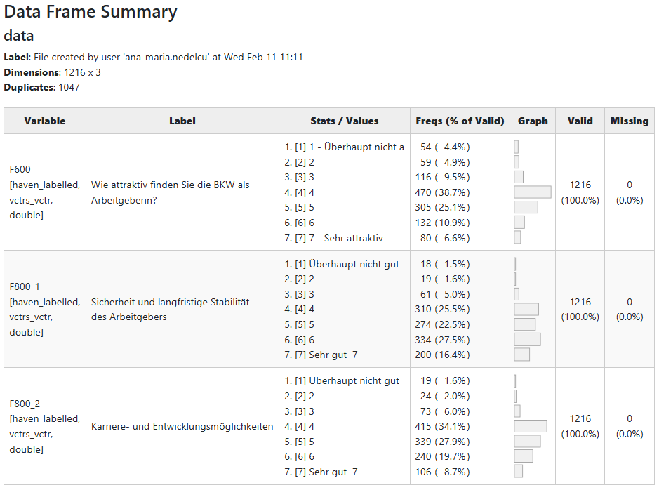
The eda_summary() function provides a comprehensive
overview of your data:
- It generates a data frame summary that displays for each variable the variable label, value labels, frquencies by values, a histogram, number of valid values and number of missing values.
- It also computes descriptive statistics for each variable: Mean, Standard Deviation, Range, Quartiles, Skewness, and Kurtosis.
By default, eda_summary() opens a browser window to
display the summary table and prints the descriptive statistics in the
console. You can control this behavior with the
console_output and browser_output
arguments.
# Provide summary in console only:
eda_summary(
  data = bkw_processed,
  variables = c("F600", "F800_1", "F800_2"), # If NULL (default), all variables are included
  console_output = TRUE,
  browser_output = FALSE
)
#> Warning: no DISPLAY variable so Tk is not available
#> Warning in png(png_loc <- tempfile(fileext = ".png"), width = 150 *
#> graph.magnif, : unable to open connection to X11 display ''
#> Warning in png(png_loc <- tempfile(fileext = ".png"), width = 150 *
#> graph.magnif, : unable to open connection to X11 display ''
#> Warning in png(png_loc <- tempfile(fileext = ".png"), width = 150 *
#> graph.magnif, : unable to open connection to X11 display ''
#>
#> ── Data Frame Summary
#> Data Frame Summary
#> data
#> Dimensions: 1171 x 3
#> Duplicates: 1013
#>
#> -------------------------------------------------------------------------------------------------------------------------------------------------
#> Variable           Label                                     Stats / Values                 Freqs (% of Valid)   Graph       Valid      Missing
#> ------------------ ----------------------------------------- ------------------------------ -------------------- ----------- ---------- ---------
#> F600               Wie attraktiv finden Sie die BKW als      1. [1] 1 - Überhaupt nicht a    43 ( 3.7%)                      1171       0
#> [haven_labelled,   Arbeitgeberin?                            2. [2] 2                        50 ( 4.3%)                      (100.0%)   (0.0%)
#> vctrs_vctr,                                                  3. [3] 3                       130 (11.1%)          II
#> double]                                                      4. [4] 4                       461 (39.4%)          IIIIIII
#>                                                              5. [5] 5                       303 (25.9%)          IIIII
#>                                                              6. [6] 6                       109 ( 9.3%)          I
#>                                                              7. [7] 7 - Sehr attraktiv       75 ( 6.4%)          I
#>
#> F800_1             Sicherheit und langfristige Stabilität    1. [1] Überhaupt nicht gut      11 ( 0.9%)                      1171       0
#> [haven_labelled,   des Arbeitgebers                          2. [2] 2                        19 ( 1.6%)                      (100.0%)   (0.0%)
#> vctrs_vctr,                                                  3. [3] 3                        66 ( 5.6%)          I
#> double]                                                      4. [4] 4                       301 (25.7%)          IIIII
#>                                                              5. [5] 5                       270 (23.1%)          IIII
#>                                                              6. [6] 6                       322 (27.5%)          IIIII
#>                                                              7. [7] Sehr gut  7             182 (15.5%)          III
#>
#> F800_2             Karriere- und Entwicklungsmöglichkeiten   1. [1] Überhaupt nicht gut      11 ( 0.9%)                      1171       0
#> [haven_labelled,                                             2. [2] 2                        34 ( 2.9%)                      (100.0%)   (0.0%)
#> vctrs_vctr,                                                  3. [3] 3                        70 ( 6.0%)          I
#> double]                                                      4. [4] 4                       417 (35.6%)          IIIIIII
#>                                                              5. [5] 5                       316 (27.0%)          IIIII
#>                                                              6. [6] 6                       234 (20.0%)          III
#>                                                              7. [7] Sehr gut  7              89 ( 7.6%)          I
#> -------------------------------------------------------------------------------------------------------------------------------------------------
#>
#> ── Descriptive Statistics
#> Variable | Mean |   SD |        Range |  Quartiles | Skewness | Kurtosis |    n | n_Missing
#> -------------------------------------------------------------------------------------------
#> F600     | 4.33 | 1.31 | [1.00, 7.00] | 4.00, 5.00 |    -0.20 |     0.48 | 1171 |         0
#> F800_1   | 5.13 | 1.29 | [1.00, 7.00] | 4.00, 6.00 |    -0.41 |    -0.11 | 1171 |         0
#> F800_2   | 4.75 | 1.20 | [1.00, 7.00] | 4.00, 6.00 |    -0.18 |     0.16 | 1171 |         0
If browser_output is set to TRUE, the
summary table looks like this:
2. Variable Correlations
The eda_correlations() function computes and visualizes
the correlation matrix for a set of variables. It supports different
correlation methods (e.g., Pearson, Spearman) and provides a heatmap
visualization of the correlations.
out <- eda_correlation(
  data = bkw_processed,
  variables = c("F600", paste0("F800_", 1:8)), # If NULL (default), all variables are included
  correlation_type = "pearson"
)

# Inspect pairwise correlations
out$d
#> # Correlation Matrix (pearson-method)
#>
#> Parameter1 | Parameter2 |    r |       95% CI | t(1169) |         p
#> -------------------------------------------------------------------
#> F600       |     F800_1 | 0.34 | [0.29, 0.39] |   12.43 | < .001***
#> F600       |     F800_2 | 0.44 | [0.39, 0.48] |   16.68 | < .001***
#> F600       |     F800_3 | 0.41 | [0.37, 0.46] |   15.58 | < .001***
#> F600       |     F800_4 | 0.47 | [0.42, 0.51] |   18.21 | < .001***
#> F600       |     F800_5 | 0.43 | [0.38, 0.48] |   16.36 | < .001***
#> F600       |     F800_6 | 0.37 | [0.32, 0.42] |   13.58 | < .001***
#> F600       |     F800_7 | 0.42 | [0.37, 0.46] |   15.66 | < .001***
#> F600       |     F800_8 | 0.45 | [0.40, 0.49] |   17.12 | < .001***
#> F800_1     |     F800_2 | 0.56 | [0.52, 0.60] |   23.25 | < .001***
#> F800_1     |     F800_3 | 0.61 | [0.57, 0.64] |   26.16 | < .001***
#> F800_1     |     F800_4 | 0.54 | [0.50, 0.58] |   21.99 | < .001***
#> F800_1     |     F800_5 | 0.51 | [0.46, 0.55] |   20.13 | < .001***
#> F800_1     |     F800_6 | 0.55 | [0.51, 0.59] |   22.57 | < .001***
#> F800_1     |     F800_7 | 0.50 | [0.45, 0.54] |   19.69 | < .001***
#> F800_1     |     F800_8 | 0.52 | [0.48, 0.56] |   20.91 | < .001***
#> F800_2     |     F800_3 | 0.54 | [0.50, 0.58] |   21.98 | < .001***
#> F800_2     |     F800_4 | 0.60 | [0.56, 0.63] |   25.57 | < .001***
#> F800_2     |     F800_5 | 0.54 | [0.50, 0.58] |   22.11 | < .001***
#> F800_2     |     F800_6 | 0.66 | [0.62, 0.69] |   29.66 | < .001***
#> F800_2     |     F800_7 | 0.65 | [0.62, 0.68] |   29.49 | < .001***
#> F800_2     |     F800_8 | 0.56 | [0.52, 0.60] |   23.31 | < .001***
#> F800_3     |     F800_4 | 0.59 | [0.56, 0.63] |   25.26 | < .001***
#> F800_3     |     F800_5 | 0.51 | [0.47, 0.55] |   20.33 | < .001***
#> F800_3     |     F800_6 | 0.53 | [0.49, 0.57] |   21.62 | < .001***
#> F800_3     |     F800_7 | 0.49 | [0.44, 0.53] |   19.04 | < .001***
#> F800_3     |     F800_8 | 0.54 | [0.49, 0.57] |   21.67 | < .001***
#> F800_4     |     F800_5 | 0.58 | [0.54, 0.62] |   24.52 | < .001***
#> F800_4     |     F800_6 | 0.58 | [0.55, 0.62] |   24.65 | < .001***
#> F800_4     |     F800_7 | 0.60 | [0.56, 0.63] |   25.44 | < .001***
#> F800_4     |     F800_8 | 0.70 | [0.67, 0.73] |   33.43 | < .001***
#> F800_5     |     F800_6 | 0.53 | [0.49, 0.57] |   21.29 | < .001***
#> F800_5     |     F800_7 | 0.60 | [0.56, 0.63] |   25.50 | < .001***
#> F800_5     |     F800_8 | 0.62 | [0.59, 0.66] |   27.27 | < .001***
#> F800_6     |     F800_7 | 0.59 | [0.55, 0.63] |   24.93 | < .001***
#> F800_6     |     F800_8 | 0.57 | [0.53, 0.61] |   23.75 | < .001***
#> F800_7     |     F800_8 | 0.60 | [0.56, 0.63] |   25.48 | < .001***
#>
#> p-value adjustment method: Holm (1979)
#> Observations: 1171

# Display correlation heatmap
out$p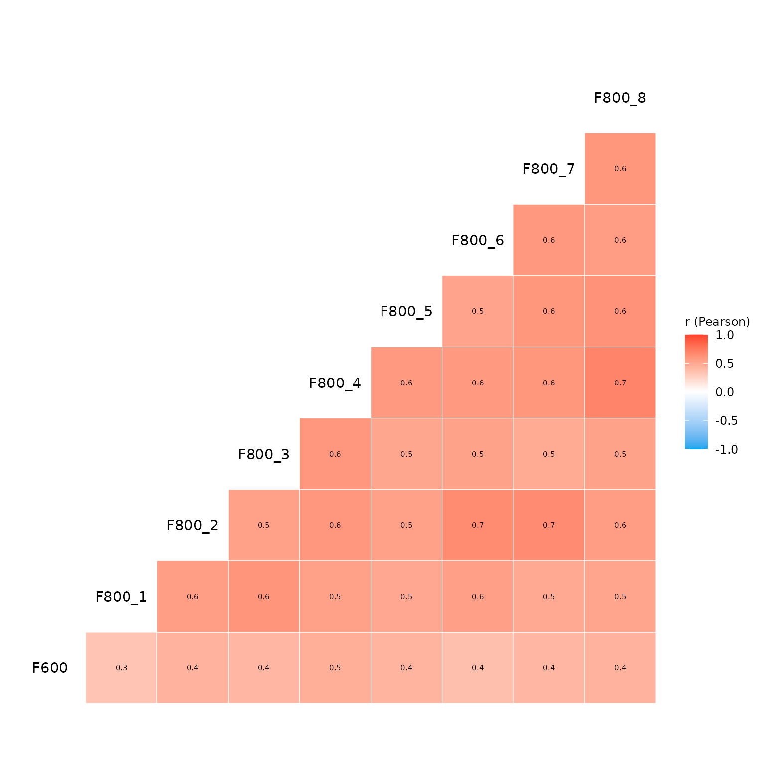
3. Going Further
If you need more sophisticated tools for EDA, I highly recommend the
package GGally, especially the function
GGally::ggpairs(), which allows you to create a matrix of
scatterplots, histograms, and correlation coefficients for a set of
variables. This can be particularly useful for visualizing relationships
between variables in your survey data.
# Create a dummy data set with a binary outcome variable coded as factor and three binary predictors
binary_data_example <- bkw_bin_outcome |>
  dplyr::select("F600", paste0("F800_", 1:3)) |>
  dplyr::mutate(F600 = haven::as_factor(F600))

# Visalize pairwise relationships with ggpairs.
GGally::ggpairs(
  data = binary_data_example,
  mapping = ggplot2::aes(color = F600)
) +
  ggplot2::scale_colour_manual(
    values = c("#ff412c", "#31caa8"),
  ) +
  ggplot2::scale_fill_manual(
    values = c("#ff412c", "#31caa8"),
  ) +
  ggplot2::theme_bw()
#> `stat_bin()` using `bins = 30`. Pick better value `binwidth`.
#> `stat_bin()` using `bins = 30`. Pick better value `binwidth`.
#> `stat_bin()` using `bins = 30`. Pick better value `binwidth`.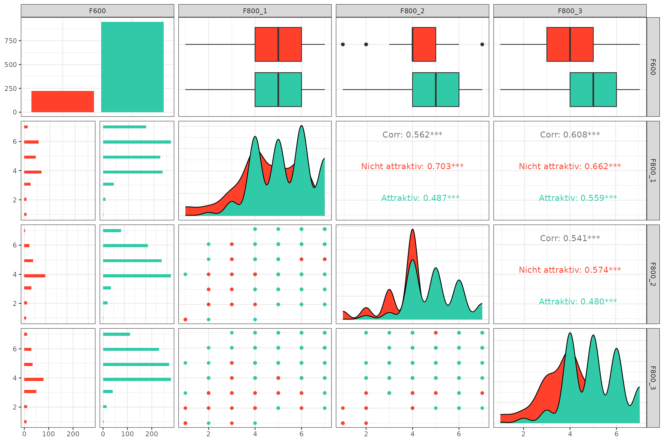
If you are using Positron as your IDE – which I cannot stress enough how much I recommend – you can also use the built-in Data Explorer, which provides a user-friendly interface for exploring your data, including summary statistics, visualizations, and the ability to filter and subset your data. Finally, also give the amazing Databot a try! It is an AI assistant that can help you with data analysis tasks, including EDA, and can be a great companion for your data analysis workflow.