Key Driver Analysis: Article • YouAnalyser

library(YouAnalyser)
#> 
#> ── Welcome to YouAnalyser! ─────────────────────────────────────────────────────
#> ✔ Package loaded successfully!
#> Type `?YouAnalyser` to see the documentation.
#> Visit the package's website for more information:
#> <https://eguizarrosales.github.io/YouAnalyser/>
library(haven)

Exploratory Data Analysis (EDA)

It is good practice to start with an exploratory data analysis (EDA) to understand the structure of the data, check for missing values, and identify any potential issues before performing Key Driver Analysis (KDA). YouAnalyser provides conventient functions for EDA, all starting with eda_: eda_summary() and eda_correlations(). These functions can help you get a quick overview of your data and identify any necessary preprocessing steps. But first, we need some data!

Reading in the data

Note that the data should be in [haven::labelled()] format for YouAnalyser to work properly, which is common for survey data. If your data is in a different format, you may need to convert it before using YouAnalyser.

We start by loading the data. The YouAnalyser package includes a sample dataset called bwk.sav, which is in SPSS format. You can read in your own dataset using the haven::read_sav() function, e.g.:

myOwnData <- haven::read_sav("path/to/your/ownFile.sav")

We can read in the included sample dataset as follows:

example_data <- haven::read_sav(system.file(
  "extdata",
  "bkw.sav",
  package = "YouAnalyser"
))

# This will be equivalent to `example_data <- YouAnalyser::bkw_missings` but using `haven::read_sav()` allows us to see how to read in our own data in the same format.

example_data contains our outcome variable F600 and 14 predictor variables F800_1 to F800_14. To get more information about this included dataset, you can run ?YouAnalyser::bkw_missings in the R console:

help(YouAnalyser::bkw_missings)

We will select only the variables of interest:

variables_of_interest <- c("F600", paste0("F800_", 1:14))
example_data <- example_data |>
  dplyr::select(all_of(variables_of_interest))

Get a summary of the data

The eda_summary() function provides a summary of the data, including the number of observations, number of missing values, and basic statistics for each variable. This can help you understand the distribution of your data and identify any potential issues.

eda_summary(example_data)

This will open a new browser window with the summary of the data that will look something like this:

#> Warning: no DISPLAY variable so Tk is not available
#> Warning in png(png_loc <- tempfile(fileext = ".png"), width = 150 *
#> graph.magnif, : unable to open connection to X11 display ''
#> Warning in png(png_loc <- tempfile(fileext = ".png"), width = 150 *
#> graph.magnif, : unable to open connection to X11 display ''
#> Warning in png(png_loc <- tempfile(fileext = ".png"), width = 150 *
#> graph.magnif, : unable to open connection to X11 display ''
#> Warning in png(png_loc <- tempfile(fileext = ".png"), width = 150 *
#> graph.magnif, : unable to open connection to X11 display ''
#> Warning in png(png_loc <- tempfile(fileext = ".png"), width = 150 *
#> graph.magnif, : unable to open connection to X11 display ''
#> Warning in png(png_loc <- tempfile(fileext = ".png"), width = 150 *
#> graph.magnif, : unable to open connection to X11 display ''
#> Warning in png(png_loc <- tempfile(fileext = ".png"), width = 150 *
#> graph.magnif, : unable to open connection to X11 display ''
#> Warning in png(png_loc <- tempfile(fileext = ".png"), width = 150 *
#> graph.magnif, : unable to open connection to X11 display ''
#> Warning in png(png_loc <- tempfile(fileext = ".png"), width = 150 *
#> graph.magnif, : unable to open connection to X11 display ''
#> Warning in png(png_loc <- tempfile(fileext = ".png"), width = 150 *
#> graph.magnif, : unable to open connection to X11 display ''
#> Warning in png(png_loc <- tempfile(fileext = ".png"), width = 150 *
#> graph.magnif, : unable to open connection to X11 display ''
#> Warning in png(png_loc <- tempfile(fileext = ".png"), width = 150 *
#> graph.magnif, : unable to open connection to X11 display ''
#> Warning in png(png_loc <- tempfile(fileext = ".png"), width = 150 *
#> graph.magnif, : unable to open connection to X11 display ''
#> Warning in png(png_loc <- tempfile(fileext = ".png"), width = 150 *
#> graph.magnif, : unable to open connection to X11 display ''
#> Warning in png(png_loc <- tempfile(fileext = ".png"), width = 150 *
#> graph.magnif, : unable to open connection to X11 display ''
#> Warning in png(png_loc <- tempfile(fileext = ".png"), width = 150 *
#> graph.magnif, : unable to open connection to X11 display ''
#> Warning in png(png_loc <- tempfile(fileext = ".png"), width = 150 *
#> graph.magnif, : unable to open connection to X11 display ''
#> Warning in png(png_loc <- tempfile(fileext = ".png"), width = 150 *
#> graph.magnif, : unable to open connection to X11 display ''
#> Warning in png(png_loc <- tempfile(fileext = ".png"), width = 150 *
#> graph.magnif, : unable to open connection to X11 display ''
#> Warning in png(png_loc <- tempfile(fileext = ".png"), width = 150 *
#> graph.magnif, : unable to open connection to X11 display ''
#> Warning in png(png_loc <- tempfile(fileext = ".png"), width = 150 *
#> graph.magnif, : unable to open connection to X11 display ''
#> Warning in png(png_loc <- tempfile(fileext = ".png"), width = 150 *
#> graph.magnif, : unable to open connection to X11 display ''
#> Warning in png(png_loc <- tempfile(fileext = ".png"), width = 150 *
#> graph.magnif, : unable to open connection to X11 display ''
#> Warning in png(png_loc <- tempfile(fileext = ".png"), width = 150 *
#> graph.magnif, : unable to open connection to X11 display ''
#> Warning in png(png_loc <- tempfile(fileext = ".png"), width = 150 *
#> graph.magnif, : unable to open connection to X11 display ''
#> Warning in png(png_loc <- tempfile(fileext = ".png"), width = 150 *
#> graph.magnif, : unable to open connection to X11 display ''
#> Warning in png(png_loc <- tempfile(fileext = ".png"), width = 150 *
#> graph.magnif, : unable to open connection to X11 display ''
#> Warning in png(png_loc <- tempfile(fileext = ".png"), width = 150 *
#> graph.magnif, : unable to open connection to X11 display ''
#> Warning in png(png_loc <- tempfile(fileext = ".png"), width = 150 *
#> graph.magnif, : unable to open connection to X11 display ''
#> Warning in png(png_loc <- tempfile(fileext = ".png"), width = 150 *
#> graph.magnif, : unable to open connection to X11 display ''

Variable

Label

Stats / Values

Freqs (% of Valid)

Graph

Missing

F600 [haven_labelled, vctrs_vctr, double]

Wie attraktiv finden Sie die BKW als Arbeitgeberin?

1. [1] 1 - Überhaupt nicht a

2. [2] 2

3. [3] 3

4. [4] 4

5. [5] 5

6. [6] 6

7. [7] 7 - Sehr attraktiv

44	(	3.6%	)
50	(	4.1%	)
132	(	10.9%	)
474	(	39.0%	)
313	(	25.8%	)
117	(	9.6%	)
84	(	6.9%	)

2 (0.2%)

F800_1 [haven_labelled, vctrs_vctr, double]

Sicherheit und langfristige Stabilität des Arbeitgebers

1. [1] Überhaupt nicht gut

2. [2] 2

3. [3] 3

4. [4] 4

5. [5] 5

6. [6] 6

7. [7] Sehr gut 7

11	(	0.9%	)
21	(	1.7%	)
67	(	5.5%	)
304	(	25.0%	)
277	(	22.8%	)
340	(	28.0%	)
195	(	16.0%	)

1 (0.1%)

F800_2 [haven_labelled, vctrs_vctr, double]

Karriere- und Entwicklungsmöglichkeiten

1. [1] Überhaupt nicht gut

2. [2] 2

3. [3] 3

4. [4] 4

5. [5] 5

6. [6] 6

7. [7] Sehr gut 7

11	(	0.9%	)
34	(	2.8%	)
70	(	5.8%	)
420	(	34.7%	)
331	(	27.3%	)
247	(	20.4%	)
98	(	8.1%	)

5 (0.4%)

F800_3 [haven_labelled, vctrs_vctr, double]

Sinnvolle Tätigkeit und gesellschaftlicher Beitrag

1. [1] Überhaupt nicht gut

2. [2] 2

3. [3] 3

4. [4] 4

5. [5] 5

6. [6] 6

7. [7] Sehr gut 7

12	(	1.0%	)
27	(	2.2%	)
91	(	7.5%	)
364	(	30.0%	)
312	(	25.7%	)
275	(	22.7%	)
133	(	11.0%	)

2 (0.2%)

F800_4 [haven_labelled, vctrs_vctr, double]

Gute Zusammenarbeit und Teamkultur

1. [1] Überhaupt nicht gut

2. [2] 2

3. [3] 3

4. [4] 4

5. [5] 5

6. [6] 6

7. [7] Sehr gut 7

13	(	1.1%	)
21	(	1.7%	)
82	(	6.7%	)
469	(	38.6%	)
337	(	27.7%	)
207	(	17.0%	)
86	(	7.1%	)

1 (0.1%)

F800_5 [haven_labelled, vctrs_vctr, double]

Vereinbarkeit von Beruf und Privatleben

1. [1] Überhaupt nicht gut

2. [2] 2

3. [3] 3

4. [4] 4

5. [5] 5

6. [6] 6

7. [7] Sehr gut 7

14	(	1.2%	)
28	(	2.3%	)
105	(	8.7%	)
451	(	37.2%	)
316	(	26.1%	)
193	(	15.9%	)
106	(	8.7%	)

3 (0.2%)

F800_6 [haven_labelled, vctrs_vctr, double]

Moderne Arbeitsumgebung und Technologien

1. [1] Überhaupt nicht gut

2. [2] 2

3. [3] 3

4. [4] 4

5. [5] 5

6. [6] 6

7. [7] Sehr gut 7

14	(	1.2%	)
26	(	2.1%	)
67	(	5.5%	)
325	(	26.8%	)
340	(	28.1%	)
286	(	23.6%	)
153	(	12.6%	)

5 (0.4%)

F800_7 [haven_labelled, vctrs_vctr, double]

Attraktive Vergütung und Zusatzleistungen

1. [1] Überhaupt nicht gut

2. [2] 2

3. [3] 3

4. [4] 4

5. [5] 5

6. [6] 6

7. [7] Sehr gut 7

13	(	1.1%	)
18	(	1.5%	)
82	(	6.8%	)
446	(	36.8%	)
293	(	24.2%	)
240	(	19.8%	)
120	(	9.9%	)

4 (0.3%)

F800_8 [haven_labelled, vctrs_vctr, double]

Gute Führung und wertschätzende Unternehmenskultur

1. [1] Überhaupt nicht gut

2. [2] 2

3. [3] 3

4. [4] 4

5. [5] 5

6. [6] 6

7. [7] Sehr gut 7

16	(	1.3%	)
32	(	2.6%	)
98	(	8.1%	)
472	(	38.9%	)
315	(	25.9%	)
189	(	15.6%	)
92	(	7.6%	)

2 (0.2%)

F800_9 [haven_labelled, vctrs_vctr, double]

Verantwortung und Gestaltungsspielraum

1. [1] Überhaupt nicht gut

2. [2] 2

3. [3] 3

4. [4] 4

5. [5] 5

6. [6] 6

7. [7] Sehr gut 7

22	(	1.8%	)
19	(	1.6%	)
120	(	9.9%	)
460	(	37.9%	)
307	(	25.3%	)
190	(	15.7%	)
95	(	7.8%	)

3 (0.2%)

F800_10 [haven_labelled, vctrs_vctr, double]

Zukunftsorientierung und Nachhaltigkeit des Unternehmens

1. [1] Überhaupt nicht gut

2. [2] 2

3. [3] 3

4. [4] 4

5. [5] 5

6. [6] 6

7. [7] Sehr gut 7

22	(	1.8%	)
20	(	1.6%	)
65	(	5.4%	)
325	(	26.8%	)
333	(	27.5%	)
324	(	26.7%	)
124	(	10.2%	)

3 (0.2%)

F800_11 [haven_labelled, vctrs_vctr, double]

Internationales Arbeitsumfeld und kulturelle Vielfalt

1. [1] Überhaupt nicht gut

2. [2] 2

3. [3] 3

4. [4] 4

5. [5] 5

6. [6] 6

7. [7] Sehr gut 7

27	(	2.2%	)
75	(	6.2%	)
156	(	12.9%	)
391	(	32.3%	)
268	(	22.1%	)
193	(	15.9%	)
101	(	8.3%	)

5 (0.4%)

F800_12 [haven_labelled, vctrs_vctr, double]

Innovationskultur und Veränderungsbereitschaft des Unternehmens

1. [1] Überhaupt nicht gut

2. [2] 2

3. [3] 3

4. [4] 4

5. [5] 5

6. [6] 6

7. [7] Sehr gut 7

18	(	1.5%	)
27	(	2.2%	)
116	(	9.6%	)
413	(	34.0%	)
333	(	27.4%	)
211	(	17.4%	)
96	(	7.9%	)

2 (0.2%)

F800_13 [haven_labelled, vctrs_vctr, double]

Arbeitszeit- und Arbeitsortflexibilität

1. [1] Überhaupt nicht gut

2. [2] 2

3. [3] 3

4. [4] 4

5. [5] 5

6. [6] 6

7. [7] Sehr gut 7

12	(	1.0%	)
32	(	2.6%	)
114	(	9.4%	)
425	(	35.0%	)
336	(	27.7%	)
199	(	16.4%	)
97	(	8.0%	)

1 (0.1%)

F800_14 [haven_labelled, vctrs_vctr, double]

Diversität, Gleichstellung und Inklusion

1. [1] Überhaupt nicht gut

2. [2] 2

3. [3] 3

4. [4] 4

5. [5] 5

6. [6] 6

7. [7] Sehr gut 7

34	(	2.8%	)
47	(	3.9%	)
94	(	7.8%	)
471	(	38.9%	)
326	(	26.9%	)
169	(	14.0%	)
69	(	5.7%	)

6 (0.5%)

Generated by summarytools 1.1.5 (R version 4.6.0)
2026-04-28

We see that there are 4307 missing values in the outcome and predictor variables. Lets remove these missing values and save the new dataset as example_data_clean:

example_data_clean <- example_data |>
  tidyr::drop_na()

Check correlations

We can also have a look at the correlation matrix of the variables using the eda_correlations() function. This can help you identify any potential multicollinearity issues among the independent variables as well as the strength and directionof the relationships between the independent variables and the dependent variable. High correlations among independent variables can indicate multicollinearity, which can affect the stability and interpretability of the KDA results. Moreover, we would like to see that the independent variables are correlated positivly with the dependent variable, as KDA is based on the idea of identifying key drivers that have a positive impact on the outcome.

corrs <- eda_correlation(example_data_clean, correlation_type = "pearson")

A correlation matrix plot is saved in corrs$p, which will look like this:

corrs$p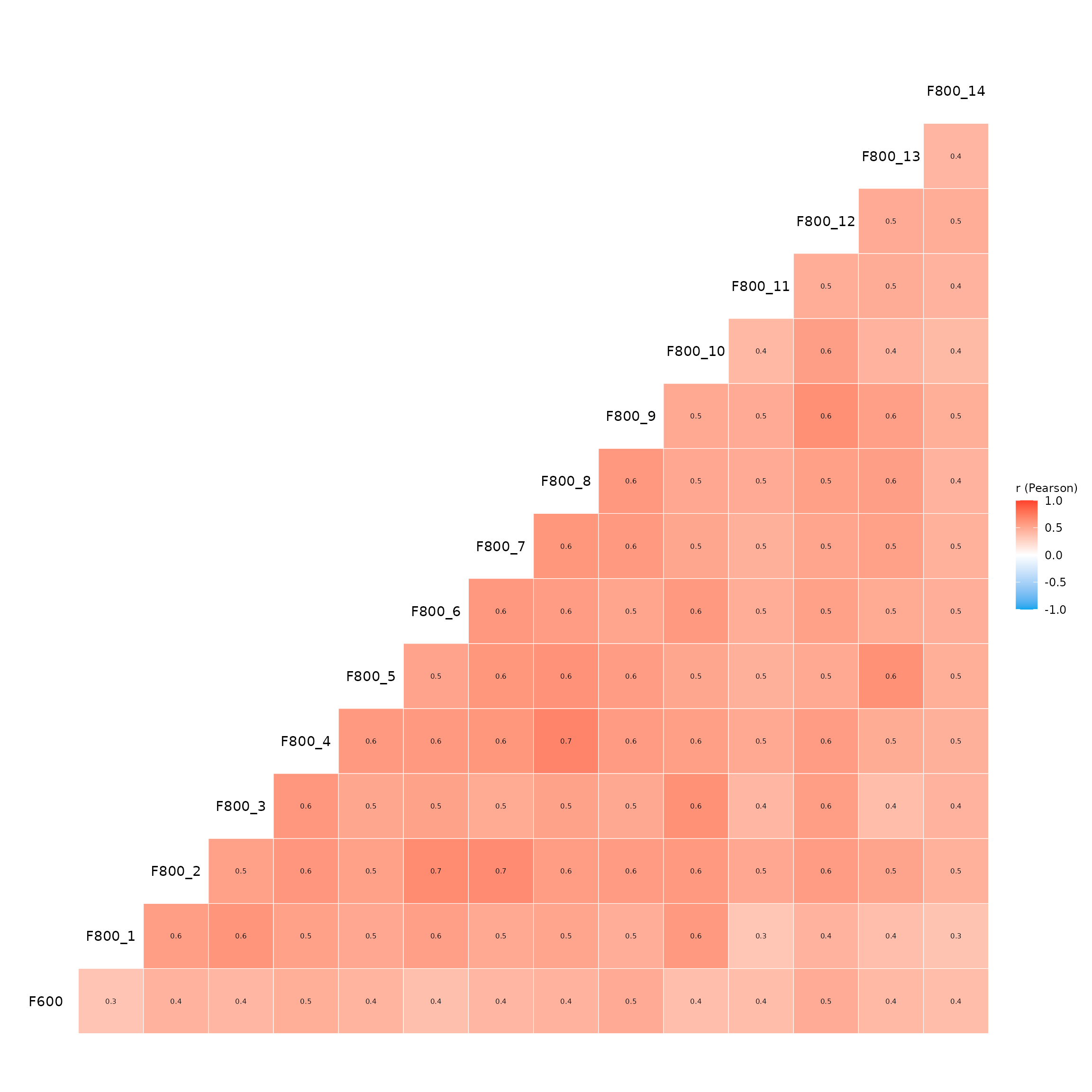

We see that there are some high correlations among the independent variables, which may indicate multicollinearity. However, we also see that all independent variables are positively correlated with the dependent variable F600, which is a good sign for performing KDA.

Key Driver Analysis (KDA)

Now the real fun starts! [YouAnalyser::kda_regression()] is the main function for performing Key Driver Analysis. There are two ways to use this function: (1) by providing the raw data and specifying the outcome variable and predictor variables, or (2) by providing a fitted model object. The first approach is more straightforward and is recommended for most users, while the second approach allows more advanced users to use some shortcuts, as we will show below.

The recommended approach in its minimal form looks like this:

kda <- kda_regression(
  data = example_data_clean,
  outcome = "F600",
  predictors = paste0("F800_", 1:14)
)

Alternatively, we can first fit a model and then provide the fitted model object to [YouAnalyser::kda_regression()]. This for instance allows for short cuts like outcome ~ . in the model formula. If you do not recognize this syntax, it is perfectly fine to ignore it and use the first approach as shown above. The second approach would look like this:

myModel <- lm(F600 ~ ., data = example_data_clean)
kda <- kda_regression(model = myModel)

Note that it is only possible to use models fitted with lm() and glm() without interaction terms! (Interactions make it very difficult to calculate usefull importance measures for KDA).

It is highly recommended to have a look at the help documentation of [YouAnalyser::kda_regression()] to see all the different options for performing KDA, including different methods for calculating importance measures and different ways to visualize the results as well as all the available output. You can access the help documentation by running ?YouAnalyser::kda_regression in the R console.

Let’s have a look at the different outputs generated by [YouAnalyser::kda_regression()]: